Blog

  • cmake-cython-example

    Example: Building C library with Cython Wrapper using CMake

    GitHub Travis (.com) Codecov

    About

    This repository shows how to use cmake to build a native C or C++ library and (optionally) add a reusable Python 3 wrapper on top using cython.

    It further shows how to use cython to implement a C interface (definition from .h file).

    Build and Run the Code

    The build uses cmake to build both the native library as well as the Python 3 bindings.

    Dependencies

    As the build uses cmake first off you will need cmake (duh).

    Additionally you will need a C compiler supporting at least C99 as well as a C++ compiler supporting at least C++11. The build should work on any compiler but was tested with gcc, clang and msbuild.

    For both the Python implementation as well as the bindings you will need to install a CPython interpreter supporting at least language level 3.6 alongside its dev tools.

    On top of that you will need to install cython to transpile the provided .pyx files to c++ and have them compiled for use in either native code or Python. For the Python tests you will need to install pytest. By default Python’s build script will check if the requirements are installed and if not install them on the fly.

    If you want to further get test coverage information for the native tests you will also need lcov.

    Finally if you also want to build the API documentation you will need doxygen for the native library as well as sphinx for the Python bindings.

    On Debian based systems you can install the required packages using:

    sudo apt-get update
    # Install required dependencies
    sudo apt-get install build-essential \
                         cmake \
                         gcc \
                         g++
    
    # Install optional dependencies
    sudo apt-get install python3 \
                         python3-dev \
                         cython3 \
                         python3-pytest \
                         python3-pytest-runner \
                         doxygen \
                         python3-sphinx \
                         lcov

    Otherwise all tools should also provide installers for your targeted operating system. Just follow the instructions on the tools’ sites.

    Build

    The build can be triggered like any other cmake project.

    cmake ..
    cmake --build .

    It offers several configuration parameters described in the following sections. For your convenience a cmake variants file is provided that lets you choose the desired target configuration.

    Library Implementation

    The library’s C API offers two different implementations:

    • The native implementation is written in pure C. This matches the typical scenario when trying to consume a native library from Python.
    • The python implementation is written in Cython. Have a look at this implementation if you want to consume Python functionality in your native C or C++ applications.

    You can choose which version to build by setting the IMPLEMENTATION cmake parameter to either native or python (default: native).

    cmake -DIMPLEMENTATION=python ..
    cmake --build .

    Python Bindings

    To enable the build of the Python bindings set the BUILD_PYTHON_BINDINGS cmake parameter to ON.

    cmake -DBUILD_PYTHON_BINDINGS=ON ..
    cmake --build .

    This will set the required configuration parameters for the Python build by generating a setup.cfg file based on the in- and output directories of the native library. The Python build can also work without cmake but you will need to make sure that Python can find the public headers for the foo library as well as the built library itself (e.g. by installing the native library).

    Depending on the other cmake settings, enabling the Python build might also enable additional features (like the sphinx based API documentation if BUILD_DOCUMENTATION is set to ON).

    Tests

    Both the native library as well as the Python bindings are unittested. To enable the automatic build of the unittests you can set the cmake parameter BUILD_TESTING to ON. After this you can run the tests by using ctest.

    cmake --build .
    ctest .

    The tests for the native library are using catch2 (provided in tests/catch2). The source code for the tests can be found in tests.

    The Python bindings use pytest. The code can be found in extras/python-bindings/tests.

    Coverage

    If you want to to get detailed information about the code coverage of the native test cases you can turn on the cmake configuration option CODE_COVERAGE (OFF by default). This option is only available if BUILD_TESTING is also enabled.

    You can then use lcov to get detailed information.

    # Build and run tests
    cmake -DBUILD_TESTING=ON -DCODE_COVERAGE=ON ..
    cmake --build .
    ctest .
    
    # Get code coverage
    lcov --capture --directory . --output-file code.coverage
    lcov --remove code.coverage '/usr/*' --output-file code.coverage
    lcov --remove code.coverage '**/tests/*' --output-file code.coverage
    lcov --remove code.coverage '**/catch.hpp' --output-file code.coverage
    lcov --list code.coverage

    Documentation

    For further information on the API you can build additional documentation yourself. Use the BUILD_DOCUMENTATION flag when configuring cmake to add the custom target documentation to the build (also added to the ALL build).

    If enabled the native API documentation will be built using doxygen and the Python documentation will be built using sphinx.

    cmake -DBUILD_DOCUMENTATION=ON ..
    cmake --build . --target documentation

    The native documentation will be put in a directory docs in cmake‘s build directory. The documentation for the Python bindings will be put in the same directory under python.

    Use Code in Own Project

    The code offers a native library that is meant to be included in your projects. To simplify the integration the repository is configured to be usable as either a (git) submodule or to be installable like any other cmake project.

    Use as (Git) Submodule

    To use the native library as a git submodule simply clone it somewhere in your source tree (e.g. in an external directory) and use add_subdirectory in your CMakeLists.txt file.

    git submodule init
    git submodule add https://github.com/kmhsonnenkind/cmake-cython-example.git external/foo

    In the CMakeLists.txt file you can then do something like:

    project(bar)
    
    add_subdirectory(external/foo)
    
    add_executable(bar bar.c)
    target_link_libraries(bar kmhsonnenkind::foo)
    

    Install to be Usable Outside of CMake

    If you want to install the native library (as well as the Python bindings) you can also use the cmake install target (might require superuser privileges):

    cmake --build .
    sudo cmake --build . --target install

    This will install:

    • The native foo library (to somewhere like /usr/local/lib/)
    • The required headers for the foo library (to somewhere like /usr/local/include/)
    • The cmake files for find_package (to somewhere like /usr/local/lib/foo/)
    • (If enabled) The Python foo package (to somewhere like /usr/local/lib/python3.6/dist-packages/)
    Visit original content creator repository https://github.com/kmhsonnenkind/cmake-cython-example
  • miknik

    Miknik


    ⚠️ Work in progress 🚧 Build Status Coverage Status

    Miknik is a temporary name which will be changed soon

    Miknik is a Mesos Framework that manages cluster capacity management automatically based on the workload. It is useful for use cases where it is hard or not practically possible to predict the workload in form of batch jobs to be scheduled for run in the Mesos cluster. Miknik will scale up your Mesos cluster by renting the resources from the cloud provider (Digital Ocean is currently supported, more planned) if number of pending jobs will exceed the configured value. It will also give the rented resources back to the cloud provider (i.e. scale cluster down) if newly rented resources keep being unused for a while.

    If you happen to know Russian, check out this ‘white paper’ (bachelor thesis) for more details: http://vital.lib.tsu.ru/vital/access/manager/Repository/vital:11294

    Currently Miknik is not production ready and should be considered a POC project. However, today it already lets you run jobs in form of docker containers with custom resource requirements that consist of CPU, memory and disk capacity.

    For usage, see HTTP API specification: http://maximskripnik.com:5161/

    Visit original content creator repository https://github.com/maximskripnik/miknik
  • contributor-role-ontology

    Build Status DOI

    Contributor Role Ontology

    The Contributor Role Ontology (CRO) is an extension of the CASRAI Contributor Roles Taxonomy (CRediT) and replaces the former Contribution Ontology.

    Versions

    Stable release versions

    The latest version of the ontology can always be found at:

    http://purl.obolibrary.org/obo/cro.owl

    (note this will not show up until the request has been approved by obofoundry.org)

    Editors’ version

    Editors of this ontology should use the edit version, src/ontology/cro-edit.owl

    Relevant publications and scholarly products

    Contact

    Please use this GitHub repository’s Issue tracker to request new terms/classes or report errors or specific concerns related to the ontology.

    Acknowledgements

    This ontology repository was created using the ontology starter kit

    Visit original content creator repository https://github.com/data2health/contributor-role-ontology
  • SneakySnake

    SneakySnake:snake:: A Fast and Accurate Universal Genome Pre-Alignment Filter for CPUs, GPUs, and FPGAs

    The first and the only pre-alignment filtering algorithm that works efficiently and fast on modern CPU, FPGA, and GPU architectures. SneakySnake greatly (by more than two orders of magnitude) expedites sequence alignment calculation for both short (Illumina) and long (ONT and PacBio) reads. Described by Alser et al. (preliminary version at https://arxiv.org/abs/1910.09020).

    💡SneakySnake now supports multithreading and pre-alignment filtering for both short (Illumina) and long (ONT and PacBio) reads

    💡Watch our lecture about SneakySnake!

    Watch our explanation of SneakySnake

    Watch our explanation of SneakySnake

    Getting Started

    git clone https://github.com/CMU-SAFARI/SneakySnake
    cd SneakySnake/SneakySnake && make
    
    #./main [DebugMode] [KmerSize] [ReadLength] [IterationNo] [ReadRefFile] [# of reads] [# of threads] [EditThreshold]
    # Short sequences
    ./main 0 100 100 100 ../Datasets/ERR240727_1_E2_30000Pairs.txt 30000 10 10
    # Long sequences
    ./main 0 20500 100000 20500 ../Datasets/LongSequences_100K_PBSIM_10Pairs.txt 10 40 20000

    Table of Contents

    The key Idea

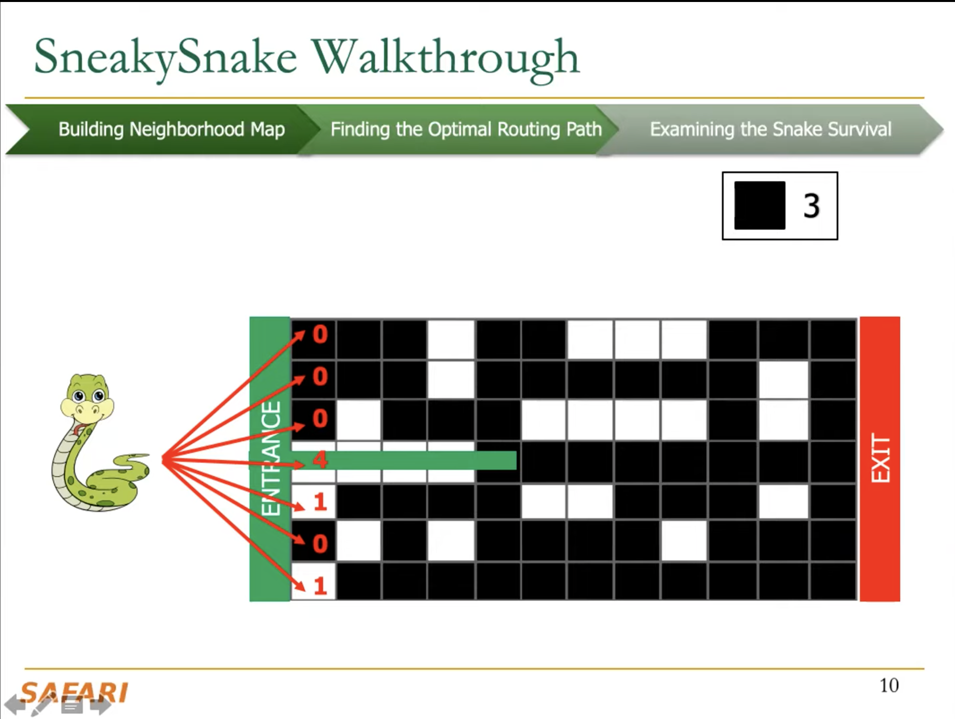
    The key idea of SneakySnake is to reduce the approximate string matching (ASM) problem to the single net routing (SNR) problem in VLSI chip layout. In the SNR problem, we are interested in only finding the optimal path that connects two terminals with the least routing cost on a special grid layout that contains obstacles. The SneakySnake algorithm quickly solves the SNR problem and uses the found optimal path to decide whether performing sequence alignment is necessary. Reducing the ASM problem into SNR also makes SneakySnake efficient to implement for modern high-performance computing architectures (CPUs, GPUs, and FPGAs).

    Benefits of SneakySnake

    SneakySnake significantly improves the accuracy of pre-alignment filtering by up to four orders of magnitude compared to the state-of-the-art pre-alignment filters, Shouji, GateKeeper, and SHD. Using short sequences, SneakySnake accelerates Edlib (state-of-the-art implementation of Myers’s bit-vector algorithm) and Parasail (sequence aligner with configurable scoring function), by up to 37.7× and 43.9× (>12× on average), respectively, without requiring hardware acceleration, and by up to 413× and 689× (>400× on average), respectively, using hardware acceleration. Using long sequences, SneakySnake accelerates Parasail by up to 979× (140.1× on average). SneakySnake also accelerates the sequence alignment of minimap2, a state-of-the-art read mapper, by up to 6.83× (4.67× on average) and 64.1× (17.1× on average) using short and long sequences, respectively, and without requiring hardware acceleration. As SneakySnake does not replace sequence alignment, users can still configure the aligner of their choice for different scoring functions, surpassing most existing efforts that aim to accelerate sequence alignment.

    Using SneakySnake:

    SneakySnake is already implemented and designed to be used for CPUs, FPGAs, and GPUs. Integrating one of these versions of SneakySnake with existing read mappers or sequence aligners requires performing three key steps: 1) preparing the input data for SneakySnake, 2) overlapping the computation time of our hardware accelerator with the data transfer time or with the computation time of the to-be-accelerated read mapper/sequence aligner, and 3) interpreting the output result of our hardware accelerator.

    1. All three versions of SneakySnake require at least two inputs: a pair of genomic sequences and an edit distance threshold. Other input parameters are the values of t and y, where t is the width of the chip maze of each subproblem and y is the number of iterations performed to solve each subproblem. Sneaky-on-Chip and Snake-on-GPU use a 2-bit encoded representation of bases packed in uint32 words. This requirement is not unique to Sneaky-on-Chip and Snake-on-GPU. Minimap2 and most hardware accelerators use a similar representation and hence this step can be opted out from the complete pipeline. If this is not the case, we already provide the script to prepare such a compact representation in our implementation. For Snake-on-Chip, it is provided in lines 187 to 193 in https://github.com/CMU-SAFARI/SneakySnake/blob/master/Snake-on-Chip/Snake-on-Chip_test.cpp and for Snake-on-GPU, it is provided in lines 650 to 710 in https://github.com/CMU-SAFARI/SneakySnake/blob/master/Snake-on-GPU/Snake-on-GPU.cu. We also observe that widely adopting efficient formats such as UCSC’s .2bit (https://genome.ucsc.edu/goldenPath/help/twoBit.html) format (instead of FASTA and FASTQ) can maximize the benefits of using hardware accelerators and reducing the resources needed to process the genomic data.
    2. The second step is left to the developer. If the developer is integrating, for example, Snake-on-Chip with an FPGA-based read mapper, then a single SneakySnake filtering unit of Snake-on-Chip (or more) can be directly integrated on the same FPGA chip, given that the FPGA resource usage of a single filtering unit is very insignificant (<1.5%). This can eliminate the need for overlapping the computation time with the data transfer time. The same thing applies when the developer integrates Snake-on-GPU with a GPU-based read mapper. The developer needs to evaluate whether utilizing the entire FPGA chip for only Snake-on-Chip (achieving more filtering) is more beneficial than combining Snake-on-Chip with an FPGA-based read mapper on the same FPGA chip.
    3. For the third step, both Sneaky-on-Chip and Snake-on-GPU return back to the developer an array that contains the filtering result (whether a sequence pair is similar or dissimilar) that appear in the same order of their original sequence pairs (input data to the first step). An array element with a value of 1 indicates that the pair of sequences at the corresponding index of the input data are similar and hence a sequence alignment is necessary.

    Directory Structure:

    SneakySnake-master
    ├───1. Datasets
    └───2. Snake-on-Chip
        └───3. Hardware_Accelerator
    ├───4. Snake-on-GPU
    ├───5. SneakySnake-HLS-HBM
    ├───6. SneakySnake
    ├───7. Evaluation Results
    
    1. In the “Datasets” directory, you will find six sample datasets that you can start with. You will also find details on how to obtain the datasets that we used in our evaluation, so that you can reproduce the exact same experimental results.
    2. In the “Snake-on-Chip” directory, you will find the verilog design files and the host application that are needed to run SneakySnake on an FPGA board. You will find the details on how to synthesize the design and program the FPGA chip in README.md.
    3. In the “Hardware_Accelerator” directory, you will find the Vivado project that is needed for the Snake-on-Chip.
    4. In the “Snake-on-GPU” directory, you will find the source code of the GPU implementation of SneakySnake. Follow the instructions provided in the README.md inside the directory to compile and execute the program. We also provide an example of how the output of Snake-on-GPU looks like.
    5. In the “SneakySnake-HLS-HBM” directory, you will find the source code of the FPGA-HBM implementation of the SneakySnake algorithm (https://arxiv.org/abs/2106.06433). Follow the instructions provided in the README.md inside the directory to compile and execute the program.
    6. In the “SneakySnake” directory, you will find the source code of the CPU implementation of the SneakySnake algorithm. Follow the instructions provided in the README.md inside the directory to compile and execute the program. We also provide an example of how the output of SneakySnake looks like using both verbose mode and silent mode.
    7. In the “Evaluation Results” directory, you will find the exact value of all evaluation results presented in the paper and many more.

    Getting Help

    If you have any suggestion for improvement, please contact mohammed dot alser at inf dot ethz dot ch If you encounter bugs or have further questions or requests, you can raise an issue at the issue page.

    Citing SneakySnake

    If you use SneakySnake in your work, please cite:

    Mohammed Alser, Taha Shahroodi, Juan Gomez-Luna, Can Alkan, and Onur Mutlu. “SneakySnake: A Fast and Accurate Universal Genome Pre-Alignment Filter for CPUs, GPUs, and FPGAs.” Bioinformatics (2020). link, link

    Gagandeep Singh, Mohammed Alser, Damla Senol Cali, Dionysios Diamantopoulos, Juan Gómez-Luna, Henk Corporaal, Onur Mutlu. “FPGA-Based Near-Memory Acceleration of Modern Data-Intensive Applications.” IEEE Micro (2021). link, link

    Below is bibtex format for citation.

    @article{10.1093/bioinformatics/btaa1015,
        author = {Alser, Mohammed and Shahroodi, Taha and Gómez-Luna, Juan and Alkan, Can and Mutlu, Onur},
        title = "{SneakySnake: a fast and accurate universal genome pre-alignment filter for CPUs, GPUs and FPGAs}",
        journal = {Bioinformatics},
        year = {2020},
        month = {12},
        abstract = "{We introduce SneakySnake, a highly parallel and highly accurate pre-alignment filter that remarkably reduces the need for computationally costly sequence alignment. The key idea of SneakySnake is to reduce the approximate string matching (ASM) problem to the single net routing (SNR) problem in VLSI chip layout. In the SNR problem, we are interested in finding the optimal path that connects two terminals with the least routing cost on a special grid layout that contains obstacles. The SneakySnake algorithm quickly solves the SNR problem and uses the found optimal path to decide whether or not performing sequence alignment is necessary. Reducing the ASM problem into SNR also makes SneakySnake efficient to implement on CPUs, GPUs and FPGAs.SneakySnake significantly improves the accuracy of pre-alignment filtering by up to four orders of magnitude compared to the state-of-the-art pre-alignment filters, Shouji, GateKeeper and SHD. For short sequences, SneakySnake accelerates Edlib (state-of-the-art implementation of Myers’s bit-vector algorithm) and Parasail (state-of-the-art sequence aligner with a configurable scoring function), by up to 37.7× and 43.9× (\\&gt;12× on average), respectively, with its CPU implementation, and by up to 413× and 689× (\\&gt;400× on average), respectively, with FPGA and GPU acceleration. For long sequences, the CPU implementation of SneakySnake accelerates Parasail and KSW2 (sequence aligner of minimap2) by up to 979× (276.9× on average) and 91.7× (31.7× on average), respectively. As SneakySnake does not replace sequence alignment, users can still obtain all capabilities (e.g. configurable scoring functions) of the aligner of their choice, unlike existing acceleration efforts that sacrifice some aligner capabilities.https://github.com/CMU-SAFARI/SneakySnake.Supplementary data are available at Bioinformatics online.}",
        issn = {1367-4803},
        doi = {10.1093/bioinformatics/btaa1015},
        url = {https://doi.org/10.1093/bioinformatics/btaa1015},
        note = {btaa1015},
        eprint = {https://academic.oup.com/bioinformatics/advance-article-pdf/doi/10.1093/bioinformatics/btaa1015/35152174/btaa1015.pdf},
    }

    Limitations

    • SneakySnake may calculate an approximated edit distance value that is very close to the actual edit distance. However, it does not over-estimate the edit distance value (i.e., its calculated edit distance is always slightly less than or equal the actual edit distance).
    Visit original content creator repository https://github.com/CMU-SAFARI/SneakySnake
  • EigenFaces

    Eigen Faces

    The following is a Demonstration of Principal Component Analysis, dimensional reduction. The following has been developed in python2.7 however can be run on machines which use Python3, by using a python virtual environment

    This project is based on the following paper:- Face recognition using eigenfaces by Matthew A. Turk and Alex P. Pentland

    Dataset courtesy – http://vis-www.cs.umass.edu/lfw/

    Development

    The following can be best developed using pipenv. If you do not have pipen, simply run the following command (using pip3 or pip based on your version of Python)

    pip install pipenv
    

    Then clone the following repository

    git clone https://github.com/sahitpj/EigenFaces
    

    Then change the following working directory and then run the following commands

    pipenv install --dev
    

    This should have installed all the necessary dependencies for the project. If the pipenv shell doesn’t start running after this, simply run the following command

    pipenv shell
    

    Now in order to run the main program run the following command

    pipenv run python main.py
    

    Make sure to use python and not python3 because the following pip environment is of Python2.7. Any changes which are to be made, are to documented and make sure to lock dependencies if dependencies have been changed during the process.

    pipenv lock
    

    The detailed report about this, can be viewd here or can be found at https://sahitpj.github.io/EigenFaces

    If you like this repository and find it useful, please consider ★ starring it 🙂

    project repo link – https://github.com/sahitpj/EigenFaces

    Principal Component Analysis

    Face Recognition using Eigen Faces – Matthew A. Turk and Alex P. Pentland

    Abstract

    In this project I would lile to demonstarte the use of Principal Component Analysis, a method of dimensional reduction in order to help us create a model for Facial Recognition. The idea is to project faces onto a feature space which best encodes them, these features spaces mathematically correspond to the eigen vector space of these vectors

    We then use the following projections along with Machine Learning techniques to build a Facial Recognizer

    We will be using Python to help us develop this model

    Introduction

    Face Structures are 2D images, which can be represented as a 3D matrix, and can be reduced to a 2D space, by converting it to a greyscale image. Since human faces have a huge amount of variations in extremely small detail shifts, it can be tough to identify to minute differences in order to distinguish people two people’s faces. Thus in order to be sure that a machine learning can acquire the best accuracy, the whole of the face must be used as a feature set.

    Thus in order to develop a Facial Recognition model which is fast, reasonably simple and is quite accurate, a method of pattern Recognition is necessary.

    Thus the main idea is to transform these images, into features images, which we shall call as Eigen Faces upon which we apply our learning techniques.

    Eigen Faces

    In order to find the necessary Eigen Faces it would be necessary to capture the vriation of the features in the face without and using this to encode our faces.

    Thus mathematically we wish to find the principal components of the distribution. However rather than taking all of the possible Eigen Faces, we choose the best faces. why? computationally better.

    Thus our images, can be represented as a linear combination of our selected eigen faces.

    Developing the Model

    Initialization

    For the followoing we first need a dataset. We use sklearn for this, and use the following lfw_people dataset. Firstly we import the sklearn library

    from sklearn.datasets import fetch_lfw_people
    

    The following datset contains images of people

    no_of_sample, height, width = lfw_people.images.shape
    data = lfw_people.data
    labels = lfw_people.target
    

    We then import the plt function in matplotlib to plot our images

    import matplotlib.pyplot as plt
    
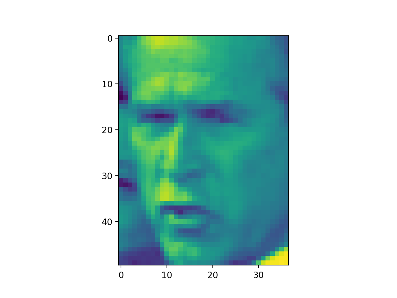
    plt.imshow(image_data[30, :, :]) #30 is the image number
    plt.show()
    

    Image 1

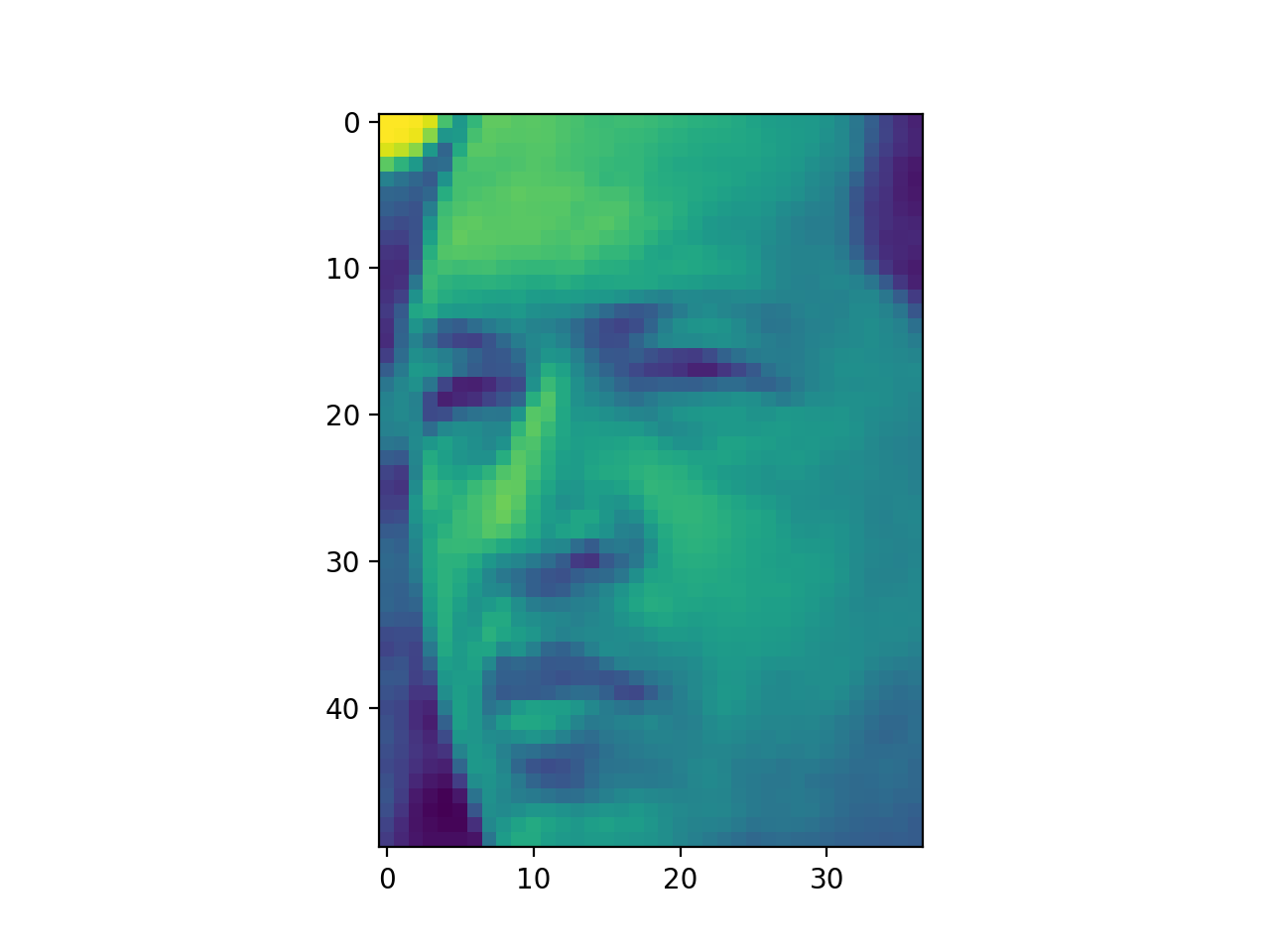
    plt.imshow(image_data[2, :, :]) 
    plt.show()
    

    Image 2

    We now understand see our labels, which come out of the form as number, each number referring to a specific person.

    jayakrishnasahit@Jayakrishna-Sahit in ~/Documents/Github/Eigenfaces on master [!?]$ python main.py
    these are the label [5 6 3 ..., 5 3 5]
    target labels ['Ariel Sharon' 'Colin Powell' 'Donald Rumsfeld' 'George W Bush'
     'Gerhard Schroeder' 'Hugo Chavez' 'Tony Blair']
    

    We now find the number of samples and the image dimensions

    jayakrishnasahit@Jayakrishna-Sahit in ~/Documents/Github/Eigenfaces on master [!?]$ python main.py
    number of images 1288
    image height and width 50 37
    

    Applying Principal Component Analysis

    Now that we have our data matrix, we now apply the Principal Component Analysis method to obtain our Eigen Face vectors. In order to do so we first need to find our eigen vectors.

    1. First we normalize our matrix, with respect to each feature. For this we use the sklearn normalize function. This subtracts the meam from the data and divides it by the variance
    from sklearn.preprocessing import normalize
    
    sk_norm = normalize(data, axis=0)
    
    1. Now that we have our data normalized we can now apply PCA. Firstly we compute the covariance matrix, which is given by
    Cov = 1/m(X'X)
    

    where m is the number of samples, X is the feature matrix and X’ is the transpose of the feature matrix. We now perform this with the help of the numpy module.

    import numpy as np 
    
    cov_matrix = matrix.T.dot(matrix)/(matrix.shape[0])
    

    the covariance matirx has dimensions of nxn, where n is the number of features of the original feature matrix.

    1. Now we simply have to find the eigen vectors of this matrix. This can be done using the followoing
    values, vectors = np.linalg.eig(cov_matrix)
    

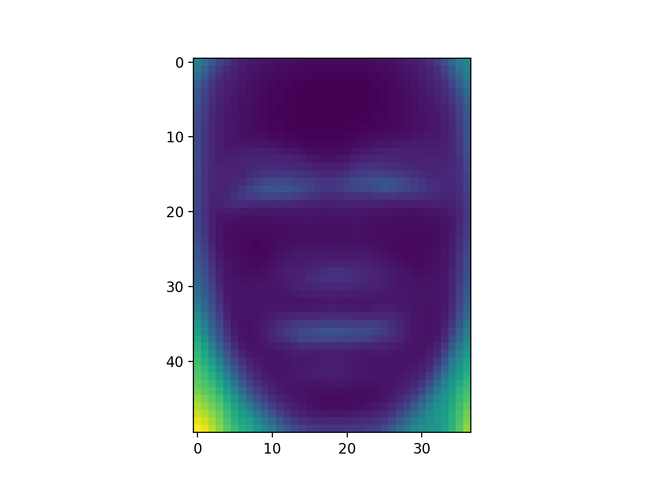
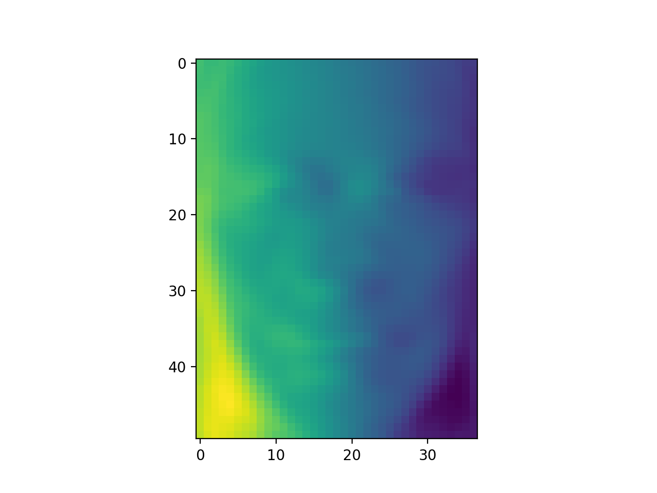
    The Eigen vectors form the Eigen Face Space and when visualised look something like this.

    Eigen Face 1

    Eigen Face 2

    Now that we have our Eigen vector space, we choose the top k number of eigen vectors. which will form our projection space.

    pca_vectors = vectors[:, :red_dim]
    

    Now in order to get our new features which have been projected on our new eigen space, we do the following

    pca_vectors = matrix.dot(eigen_faces) 
    

    We now have our PCA space ready to be used for Face Recognition

    Applying Facial Recognition

    Once we have our feature set, we now have a classification problem at our hands. In this model I will be developing a K Nearest Neighbour model (Disclaimer! – This may not be the best model to use for this dataset, the idea is to understand how to implement it)

    Using out sklearn library we split our data into train and test and then apply our training data for the Classifier.

    from sklearn.model_selection import train_test_split
    from sklearn.neighbors import KNeighborsClassifier
    
    X_train, X_test, y_train, y_test = train_test_split(pca_vectors, labels, random_state=42)
    
    knn = KNeighborsClassifier(n_neighbors=10)
    knn.fit(X_train, y_train)
    

    And we then use the trained model on the test data

    print 'accuracy', knn.score(X_test, y_test)
    
    jayakrishnasahit@Jayakrishna-Sahit in ~/Documents/Github/Eigenfaces on master [!?]$ python main.py
    accuracy 0.636645962733
    
    Visit original content creator repository https://github.com/sahitpj/EigenFaces
  • splicinglore_website

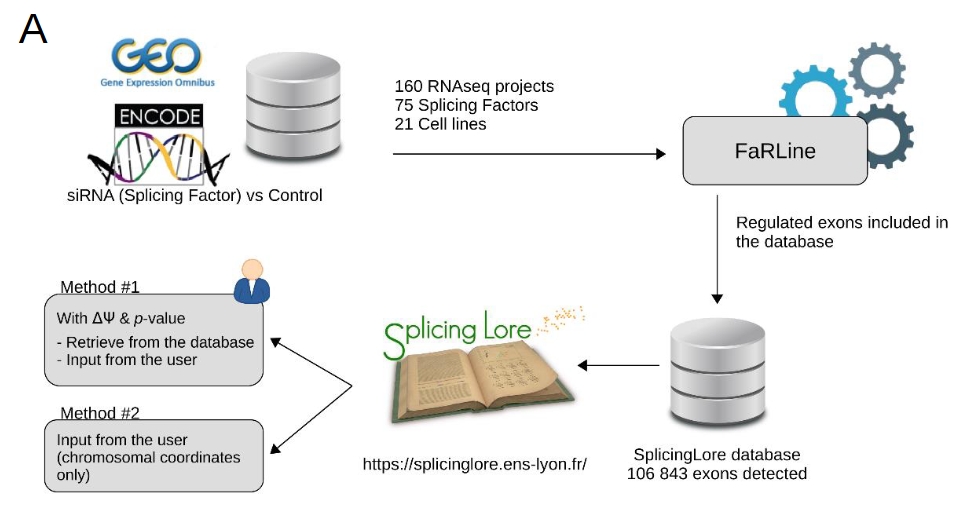
    SplicingLore: a web resource for studying the regulation of cassette exons by human splicing factors

    2023-06-30

    Helene Polveche, Jessica Valat, Nicolas Fontrodona, Audrey Lapendry, Stephane Janczarski, Franck Mortreux, Didier Auboeuf, Cyril F Bourgeois

    doi: https://doi.org/10.1101/2023.06.30.547181

    https://splicinglore.ens-lyon.fr

    Installation

    Debian

    sudo apt install libcurl4-openssl-dev libxml2-dev libssl-dev pandoc libfontconfig1-dev libharfbuzz-dev libfribidi-dev libfreetype6-dev libpng-dev libtiff5-dev libjpeg-dev librsvg2-dev libpq-dev  libudunits2-dev unixodbc-dev libproj-dev libgdal-dev libcairo2-dev libxt-dev 
    
    sudo apt install build-essential zlib1g-dev libncurses5-dev libgdbm-dev libnss3-dev libreadline-dev libffi-dev libsqlite3-dev libbz2-dev
    
    sudo apt install bedtools
    

    R packages ( 4.2 )

    install.packages("tidyverse", lib = "/usr/local/lib/R/site-library", dependencies = T) 
    install.packages("plotly", lib = "/usr/local/lib/R/site-library", dependencies = T) 
    install.packages("htmlwidgets", lib = "/usr/local/lib/R/site-library", dependencies = T) 
    
     if (!requireNamespace("BiocManager", quietly = TRUE))
       install.packages("BiocManager", lib = "/usr/local/lib/R/site-library", dependencies=T)
     BiocManager::install("rtracklayer", lib = "/usr/local/lib/R/site-library", dependencies=T)
     BiocManager::install("liftOver", lib = "/usr/local/lib/R/site-library", dependencies=T)
    

    Python ( 3.10 )

    pip3.10 install numpy panda loguru
    pip3.10 install lazyparser statsmodels rich pymysql
    
    Visit original content creator repository https://github.com/helenepolveche/splicinglore_website
  • Spectra


    Spectra logo

    A Python-based graphical interface for analyzing bacterial inhibition and generating customizable graphs.

    Spectra GUI screenshot

    Overview

    This project is part of my undergraduate thesis in Biomedical Sciences, titled “Comparative Analysis Between the Use of Oxyreductive Dye and Automated Reading in the Determination of the Minimum Inhibitory Concentration in Bacteria of Medical Importance”. It is a Python-based graphical user interface (GUI) designed to optimize experiments aimed at determining the percentage of bacterial inhibition and the Minimum Inhibitory Concentration (MIC) in 96-well microplate experiments. The data obtained is represented through customizable graphs, which can be saved in various formats. This project builds upon the findings of a previously published article.

    Features

    Key Features:

    • Bacterial Inhibition Calculation: Automatically calculates the percentage of bacterial inhibition based on absorbance values.
    • Customizable Graphs: Generates graphs that can be personalized (colors, titles, axes, etc.).
    • File Export: Allows saving graphs in formats such as .jpg, .png, .pdf, and .svg, and exporting data as .csv.
    • Interactive Table: Allows easy input of absorbance values.
    • Dynamic Graph Generation: Graphs are generated dynamically based on input data.
    • Data Processing: Handles absorbance data and calculates inhibition percentages.
    • Graph Customization: Supports customization of graph elements (e.g., colors, titles, axes).

    How to Use?

    This project was designed based on experiments conducted with Staphylococcus aureus and Escherichia coli, where each dye occupies two rows (duplicates), and the positive and negative controls occupy the last two columns of the microplate. However, it is possible to configure the position of the controls, the bacteria used, and the antibiotic concentration corresponding to the experiment. The microplate line-up used in the experiments can be found in the mentioned article.

    Steps:

    1. Select the Bacteria: Choose the bacteria used in the experiment from the options provided.
    2. Input Absorbance Values: Enter the absorbance values into the table provided in the interface. (You don’t need to fill the entire table if the experiment used fewer dyes and duplicates.)
    3. Select Duplicates: For each duplicate, select the two rows and press the button corresponding to the dye used in the duplicate.
    4. Generate Graph: After completing the input, click “Generate Graph.” The corresponding graph will automatically appear in the “Graph” tab. The graph can be customized (colors, titles, axes) and saved.

    Setup

    You can run the application in two ways: by downloading the pre-built executable or by setting up the project locally.

    Option 1: Download the Pre-built Executable

    1. Go to the Releases page.
    2. Download the .exe file from the latest release.
    3. Run the .exe file on a Windows machine.

    Option 2: Run Locally

    To run the application locally, you’ll need Git and Python installed.

    # Clone this repository
    $ git clone https://github.com/luizreinert/Spectra
    
    # Install dependencies
    
    # Run the application
    $ python Spectra.py

    Tech Stack

    License

    This project is licensed under the MIT License.


    Made with 💙 by Luiz Reinert

    Visit original content creator repository https://github.com/luizreinert/Spectra
  • gify

    GIF App

    This is a web application that allows users to search for and explore GIFs sourced from the Giphy API. It provides a user-friendly interface for discovering and sharing animated GIFs.

    Features

    • GIF Search : Search for GIFs by entering keywords or phrases.
    • Trending GIFs : Explore trending GIFs to discover popular content.
    • Random GIFs : View random GIFs for entertainment.
    • Download GIFs : Download GIFs to your device for offline use or sharing.

    Libraries and Tools used in this project

    • Reactjs (a Javscript library for building user interface ).
    • MaterialUI ( styling library sponsored by Google).
    • Axios (An Https library for fetching API data).
    • GIT (A version control system for deploying the code to Github).
    • React-Router (routing library to navigate between the web-pages).

    Usage

    To rund this project locally, follow these steps.

    1. Clone this repository.
    2. Install dependencies using npm install or Yarn Install.
    3. Start the server using npm start or Yarn start.
    4. Open your browser and navigate to http://localhost:port (replace port with the port number configured in your environment).
    5. Obtain an API key from GPIHY and replace YOUR_API_KEY in the code with my actual API key.

    Visit original content creator repository
    https://github.com/saladilakshman/gify

  • ytbulk

    YTBulk Downloader

    A robust Python tool for bulk downloading YouTube videos with proxy support, configurable resolution settings, and S3 storage integration.

    Features

    • Bulk video download from CSV lists
    • Smart proxy management with automatic testing and failover
    • Configurable video resolution settings
    • Concurrent downloads with thread pooling
    • S3 storage integration
    • Progress tracking and persistence
    • Separate video and audio download options
    • Comprehensive error handling and logging

    Installation

    1. Clone the repository
    2. Install dependencies:
    pip install -r requirements.txt

    Configuration

    Create a .env file with the following settings:

    YTBULK_MAX_RETRIES=3
    YTBULK_MAX_CONCURRENT=5
    YTBULK_ERROR_THRESHOLD=10
    YTBULK_TEST_VIDEO=<video_id>
    YTBULK_PROXY_LIST_URL=<proxy_list_url>
    YTBULK_PROXY_MIN_SPEED=1.0
    YTBULK_DEFAULT_RESOLUTION=1080p

    Configuration Options

    • YTBULK_MAX_RETRIES: Maximum retry attempts per download
    • YTBULK_MAX_CONCURRENT: Maximum concurrent downloads
    • YTBULK_ERROR_THRESHOLD: Error threshold before stopping
    • YTBULK_TEST_VIDEO: Video ID used for proxy testing
    • YTBULK_PROXY_LIST_URL: URL to fetch proxy list
    • YTBULK_PROXY_MIN_SPEED: Minimum acceptable proxy speed (MB/s)
    • YTBULK_DEFAULT_RESOLUTION: Default video resolution (360p, 480p, 720p, 1080p, 4K)

    Usage

    python -m cli CSV_FILE ID_COLUMN --work-dir WORK_DIR --bucket S3_BUCKET [OPTIONS]

    Arguments

    • CSV_FILE: Path to CSV file containing video IDs
    • ID_COLUMN: Name of the column containing YouTube video IDs
    • --work-dir: Working directory for temporary files
    • --bucket: S3 bucket name for storage
    • --max-resolution: Maximum video resolution (optional)
    • --video/--no-video: Enable/disable video download
    • --audio/--no-audio: Enable/disable audio download

    Example

    python -m cli videos.csv video_id --work-dir ./downloads --bucket my-youtube-bucket --max-resolution 720p

    Architecture

    Core Components

    1. YTBulkConfig (config.py)

      • Handles configuration loading and validation
      • Environment variable management
      • Resolution settings
    2. YTBulkProxyManager (proxies.py)

      • Manages proxy pool
      • Tests proxy performance
      • Handles proxy rotation and failover
      • Persists proxy status
    3. YTBulkStorage (storage.py)

      • Manages local and S3 storage
      • Handles file organization
      • Manages metadata
      • Tracks processed videos
    4. YTBulkDownloader (download.py)

      • Core download functionality
      • Video format selection
      • Download process management
    5. YTBulkCLI (cli.py)

      • Command-line interface
      • Progress tracking
      • Concurrent download management

    Proxy Management

    The proxy system features:

    • Automatic proxy testing
    • Speed-based verification
    • State persistence
    • Automatic failover
    • Concurrent proxy usage

    Storage System

    Files are organized in the following structure:

    work_dir/
    ├── cache/
    │   └── proxies.json
    └── downloads/
        └── {channel_id}/
            └── {video_id}/
                ├── {video_id}.mp4
                ├── {video_id}.m4a
                └── {video_id}.info.json
    

    Error Handling

    • Comprehensive error logging
    • Automatic retry mechanism
    • Proxy failover
    • File integrity verification
    • S3 upload confirmation

    Contributing

    1. Fork the repository
    2. Create a feature branch
    3. Commit your changes
    4. Push to the branch
    5. Create a Pull Request

    License

    MIT License

    Dependencies

    • yt-dlp: YouTube download functionality
    • click: Command line interface
    • python-dotenv: Environment configuration
    • tqdm: Progress bars
    • boto3: AWS S3 integration

    Visit original content creator repository
    https://github.com/storytracer/ytbulk

  • udacity_capstone_farmland_avian_dataset

    Udacity Data Engineering Capstone Project: Data Warehouse

    Farmland and Grassland Avian Ecology Data Warehouse Implementation in AWS Redshift, PostGreSQL, and Python

    Background

    The objective of this project is to compile a dataset comprised of agricultural survey data and avian sighting records for species which rely heavily on grassland and farmland ecosystems for survival. The scope of this dataset is for the year 2017 within the United States. Species included in this dataset were manually selected based on literature searches for songbirds which rely on these habitats for food, shelter, and overall survival.

    Data Selection

    NASS/NASS Census of Agriculture Data

    2017 USDA/NASS Census of Agriculture Data was acquired from NASS.USDA.gov in an Excel format. Two tables were extracted from this Excel file. The first describes various parameters of land use and chemical use on farms, and was extracted locally as a .csv file. The second was a table containing FIPS data for each county surveyed, and was extracted locally as a .json file to satisfy project requirement of two types of data sources for ingestion.

    The farms table contains metadata including Acres of Land in Farms, Acres of Irrigated Land as Percent of Land in Farms, Acres of Total Cropland as Percent of Land in Farms, Acres of Harvested Cropland as Percent of Land in Farms, Acres of Pastureland as Percent of Land in Farms, Acres Enrolled in Conservation Reserve, Acres Treated with Chemicals to Control Insects, Acres Treated with Chemicals to Control Nematodes, Acres Treated with Chemicals to Contorl Weeds, Acres Treated with Chemicals to Control Growth, Acres Treated with Chemicals to Control Disease. Each of these was encoded with a value provided by NASS in the foramt y17_Mxxx. Mapping is described in the data dicitonary.

    eBird Data

    eBird data was acquired by request at https://ebird.org/science/use-ebird-data. Requests were made for 17 species of songbird, with parameters of Country = ‘United States’ and date between Jan 2017 and Dec 2017. Data was acquired for the below species:

    ‘Northern Bobwhite’, ‘Horned Lark’, ‘Upland Sandpiper’, ‘Grasshopper Sparrow’ “Baird’s Sparrow” ‘Long-billed Curlew’, ‘American Pipit’ ‘Killdeer’ “Sprague’s Pipit” ‘Lapland Longspur’, ‘Vesper Sparrow’, ‘House Sparrow’, ‘Red-winged Blackbird’, ‘Bobolink’, ‘Snow Bunting’, ‘Song Sparrow’, ‘Eastern Meadowlark’

    Quality checks were run on the data to ensure that the species list in the raw dataset was curated into a proper controlled vocabulary, and that the dates were within the designated dates for the project. These quality checks can be found in the eBird_data_acquisition.py script.

    Data Model

    An image of the data model is provided in this repository. It follows the format below:

    Fact Table: Observation_table

    • observation_id PRIMARY KEY INT
    • common_name TEXT
    • FIPS_code INT
    • observation_count TEXT
    • sampling_event_id TEXT
      note about observation_count – while in an analysis this would be ideal as an integer,
      there are cases where the reporter of the sighting could not define ane exact count of a species
      due to a large flock or uncertainty if the same bird was seen multiple times. These are reported as ‘X’.
      Rather than attempt to impute during this dataset construction, I would leave this imputation up to
      the data scientist or analyst executing the downstream analytics in this case.

    Dimension Table: FIPS_table

    • FIPS_code PRIMARY KEY INT
    • county TEXT
    • state TEXT

    Dimension Table: Farm_table
    -FIPS_code PRIMARY KEY INT
    -y17_M059 TEXT
    -y17_M061 TEXT
    -y17_M063 TEXT
    -y17_M066 TEXT
    -y17_M068 TEXT
    -y17_M070 TEXT
    -y17_M078 TEXT
    -y17_M079 TEXT
    -y17_M080 TEXT
    -y17_M081 TEXT
    -y17_M082 TEXT
    note – variable meaning described in data dictionary, too long for column headers

    Dimension Table: Sampling_event_metadata_table
    sampling_event_id TEXT PRIMARY KEY
    locality TEXT
    latitude FLOAT
    longitude FLOAT
    observation_date TEXT
    observer_id TEXT
    duration_minutes INT
    effort_distance_km INT

    Dimension Table: Taxonomy
    common_name TEXT PRIMARY KEY
    scientific_name TEXT
    taxonomic_order TEXT

    The model was constructed by executing the following steps:

    1. NASS/USDA data acquistion script execution to output two files: Farms.csv and FIPS.json (input for ETL – two data source types).
    2. A .csv file for each of the 17 species listed above. An eBird data acquisition script was run to append, clean, and output a merged_cleaned.csv file.
    3. All three of the output files were inserted into an S3 bucket, which is the input source for the ETL project dataset.
    4. A create_tables script was run to execute SQL queries in PostgreSQL to create the tables in Redshift.
    5. The ETL.py script was run to execute staging table creation, copying into staging tables, and execution of data insert into the Redshift tables.

    Use-cases and Sample Queries

    This data preparation exercise resulted in a table which could be used as either an analytics table or an application back-end. This is a static dataset from a temporal perspective since the Agricultural Census only occurs every 5 years. In theory this could be curated every 5 years to assess change.

    With respect to use-cases, this dataset could be used by ornithology researchers, policymakers, or farmers to understand the potential impact of farmland acreage, chemical use, and geography on avian populations and ecosystem dynamics. This past June, the United States passed the Growing Climate Solutions Act , which support farmers in implementing sustainable and environmentally-friendly practices, ultimately benefiting avian populations rebound from their current status. This area of sustainable agriculture is a topic of interest and this dataset could serve as a conceptual model to build upon with future census data and eBird checklists. Some sample queries have been executed in Redshift and images were pasted into a Jupyter Notebook report attached in this repository.

    To summarize scenarios which are outlined in the query report (sample_queries.pynb) attached to this repository:
    Query 1 Justification: A reasearcher wants to get the count of species observation reports (not SUM) grouped by county and state by species.
    Query 2 Justification: An ornithologist wants to track their labs sightings by seeing a list of all species observed by observer_id
    Query 3 Justification: A policymaker wants to understand how Acreage of Farmland, Cropland, and Chemical usage on farmland impacts bird populations by county and state. This could be leveraged to strengthen positions of sustainable agriculture and conservation.
    Query 4 Justification: A policymaker or researcher wants to get an idea of the amount of farmland which is part of conservation efforts or sustainable farming efforts in a given county or state to inform policy decisions or research hypotheses on species population dynamics.
    Query 5 Justification: Getting counts on all 5 tables. Project requirement: at least 1 million rows. Rows in fact table: 3.4 million.

    Data Updates, Future Scenarios, and Pipelines

    Agricultural census data is only updated every 5 years, while eBird data is constantly available. There is an eBird API which could be leveraged to access real-time data, but there are limitations to amount of data which can be extracted. If an agreement was reached with Cornell Lab of Ornithology, the export files could be provided on a yearly basis to feed a data pipeline. I would propose the following pipeline for a productionized version of this dataset, leveraging Apache Airflow:

    1. Acquire all 17 species eBird files on a yearly basis and run the eBird_data_acquisition.py to clean, append, and quality check the data.
    2. Acquire NASS/USDA Agricultural Census summary data every 5 years as it becomes available and run the NASS_data_acquisition.py to clean and sort the data.
    3. Modify ETL to handle cases of interim years where Agricultural Summary data is not available, in order to handle only eBird data.

    If the data size was increased by 100x (as proposed in project write-up scenario): leverage Spark instead of Pandas for data acquisition and writing to Redshift.

    If the pipelines were run on a daily basis at 7AM (as proposed in the project write-up scenario): This is not relevant for this scenario, however if eBird API data were theoretically to be acquired daily at 7AM, an Airflow DAG could be set up to run the API calls separately and feed the data into the eBird_data_acquisition script.

    If the database needed to be acessed by 100+ people (as proposed in project write-up scenario): Launch on RA3.16xlarge, RA3.4xlarge, or RA3.xlplus nodes in Redshift

    Data Dictionary

    Observations

    common_name common: (non-scientific) name of species observed
    FIPS_code: FIPS code (geopgraphic information data)
    observation_date: date of eBird species observation
    sampling_event_id: unique identifier for sampling event (aka eBird checklist – can include multiple spcies, at a given location and date/time)

    Farms

    FIPS_code: FIPS code (geographic information data)
    y17_M059: Acres of Land in Farms as Percent of Land Area in Acres: 2017
    y17_M061: Acres of Irrigated Land as Percent of Land in Farms Acreage: 2017
    y17_M063: Acres of Total Cropland as Percent of Land Area in Acres: 2017
    y17_M066: Acres of Harvested Cropland as Percent of Land in Farms Acreage: 2017
    y17_M068: Acres of All Types of Pastureland as Percent of Land in Farms Acreage: 2017
    y17_M070: Acres Enrolled in the Conservation Reserve, Wetlands Reserve, Farmable Wetlands, or Conservation Reserve Enhancement Programs as Percent of Land in Farms Acreage: 2017
    y17_M078: Acres of Cropland and Pastureland Treated with Animal Manure as Percent of Total Cropland Acreage: 2017
    y17_M079: Acres Treated with Chemicals to Control Insects as Percent of Total Cropland Acreage: 2017
    y17_M080: Acres Treated with Chemicals to Control Nematodes as Percent of Total Cropland Acreage: 2017
    y17_M081: Acres of Crops Treated with Chemicals to Control Weeds, Grass, or Brush as Percent of Total Cropland Acreage: 2017
    y17_M082: Acres of Crops Treated with Chemicals to Control Growth, Thin Fruit, Ripen, or Defoliate as Percent of Total Cropland Acreage: 2017
    y17_M083: Acres Treated with Chemicals to Control Disease in Crops and Orchards as Percent of Total Cropland Acreage: 2017

    FIPS

    FIPS_code: FIPS code (geographic information data)
    county: county associated with FIPS code
    state: state associated with FIPS code

    Sampling Event Metadata

    sampling_event_id: value from eBird, unique identifier for checklist/sampling event
    locality: value from eBird, aka a ‘hotspot’, is a location defined in eBird. can be a park, hiking trail, farm, forest, roadside area, beach, etc.
    latitude: latitude
    longitude: longitude
    observation_date: date of observation via eBird
    observer_id: identifier of the birdwatcher who logged the sighting on eBird
    duration_minutes: duration of the eBird sampling event (hours spent by the birdwatcher/observer on that sampling event)
    effort_distance_km: distance traveled during the eBird sampling event by the birdwatcher/observer

    Taxonomy

    common_name: common name (non-scientific) of the species observed
    scientific_name: scientific (latin) name of the species observed
    taxonomic_order: biological classification, taxonomic classification

    References and Acknowledgements

    eBird – cornell lab of ornithology: eBird.org
    NASS/USDA: NASS.usda.gov

    Visit original content creator repository
    https://github.com/salamandersen93/udacity_capstone_farmland_avian_dataset